Making tables in a PDF using R

A guide on making tables in PDF using RMarkdown and kableExtra.
RMarkdown
kableExtra
Author

Sharleen Weatherley

Published

September 1, 2019

TL;DR

Today we will be making this in a PDF, starting from a tidy data frame of city population data:

Image of the pdf that we will be making

Introduction

As part of my job, there is a report I create every year.

Last year, I wrote the report without using R. My workflow went like this:

  • Import the CSV file into SPSS
  • Manually clean the data and create the tables
  • Paste the tables into Excel for formatting
  • Paste the tables into Word for more formatting
  • Send it to another team to professionally graphic-design the report
  • Send the PDF to be published on the website

Here is what last year’s report looked like: http://ccrnr.ca/assets/2018-nclex-rn-2017-canadian-and-international-results-ccrnr-en.pdf

I mean, it’s pretty good! But it’s not very reproducible…

Since then, at my work, we’ve been converting all of our processes to be more reproducibly written in R! This is much more efficient, and more fun!

So this year, while writing the report using R, my workflow went like this:

  • Import the CSV file into R
  • Run my .R script to clean the data
  • Run my .Rmd script to create the PDF
  • Commit any changes, because the report is now version-controlled thanks to Jenny Bryan’s Happy Git and GitHub for the useR! 😍
  • Send the PDF to be published on the website

This is much more reproducible and will make the creation of next year’s report so much faster!

Click here to see what this year’s reproducible report looked like: http://ccrnr.ca/assets/2018-ccrnr-nclex-canadian-and-international-results-report-en.pdf

How did I create the tables in PDF?

After posting on Twitter about this updated process, some people asked how I created the tables in PDF using R.

Well, the first few set-up steps in order to create tables in PDF are as follows:

  • First, I downloaded the tinytex package in R
  • I also installed the bookdown package in R, in order to be able to cross-reference tables (then the YAML output document type is bookdown::pdf_document2)
  • I also installed the knitr and kableExtra packages, in order to be able to create the tables themselves using the kable() function

🍁 A Canadian example! 🍁

Now I’ll go through an example that uses all of the techniques I used while I was writing the report!

The Wikipedia page List of the 100 largest population centres in Canada has a table containing the largest 100 population centres (“cities”) in Canada, along with their populations in 2011 and 2016.

My goal is to make a table that shows:

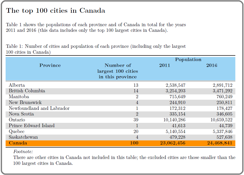
  • the number of cities in each province that are in the top 100
  • the population of each province in 2011 and 2016 (including the populations of the top 100 cities only)
  • a “Total” row for Canada that shows the total number of cities (this number should equal 100)
  • the population of Canada in 2011 and 2016 (including the populations of the top 100 cities only)

I used the website Convert Wiki Tables to CSV to turn the table on the Wikipedia page into a CSV file. Click here to see the full raw file on my Github page.

Data import

Here is the R code where I import the CSV file I created ("wiki_data.csv"). Underneath the code, I’ve displayed what the raw data file looks like.

library(dplyr)
library(janitor)
library(stringr)
library(knitr)
library(kableExtra)
library(readr)

wiki_data_raw <- read_csv(here::here("posts",
                                     "2019-09-01-tables-in-pdf",
                                     "wiki_data.csv")) %>%
  clean_names()

wiki_data_raw %>%
  head()
# A tibble: 6 × 7
   rank population_centre    province      population_in_2016 population_in_2011
  <dbl> <chr>                <chr>                      <dbl>              <dbl>
1     1 "Toronto"            Ontario                  5429524            5144412
2     2 "Montreal"           Quebec                   3519595            3387653
3     3 "Vancouver"          British Colu…            2264823            2124443
4     4 "Calgary"            Alberta                  1237656            1094379
5     5 "Edmonton"           Alberta                  1062643             935361
6     6 "Ottawa\x96Gatineau" Ontario/Queb…             989657             945592
# ℹ 2 more variables: percent_change <chr>, class <chr>

Data cleaning

I am only interested in the province of each city and what its population was in 2011 and 2016, so my first step in cleaning will be to select only those three columns. I will then use group_by and summarize to get the number of cities and populations on a per-province basis.

wiki_data_by_province <- wiki_data_raw %>%
  select(province,
         population_2016 = population_in_2016,
         population_2011 = population_in_2011) %>%
   # Since some provinces were actually two provinces put together
   # (e.g., "Alberta/Saskatchewan"), I used regex code from this website
   # (https://www.perlmonks.org/?node_id=908348) to get everything before
   # the first forward slash in the string
  mutate(province = str_extract(province, "^([^\\/]+)")) %>%
  group_by(province) %>%
  summarize(number_of_cities_in_top_100 = n(),
            pop_of_largest_cities_2011 = sum(population_2011),
            pop_of_largest_cities_2016 = sum(population_2016))

wiki_data_by_province
# A tibble: 10 × 4
   province number_of_cities_in_…¹ pop_of_largest_citie…² pop_of_largest_citie…³
   <chr>                     <int>                  <dbl>                  <dbl>
 1 Alberta                      13                2538547                2891712
 2 British…                     14                3254203                3471292
 3 Manitoba                      2                 715649                 760249
 4 New Bru…                      4                 244910                 250811
 5 Newfoun…                      1                 172312                 178427
 6 Nova Sc…                      2                 335154                 346605
 7 Ontario                      39               10140286               10659522
 8 Prince …                      1                  41613                  44739
 9 Quebec                       20                5140554                5337846
10 Saskatc…                      4                 479228                 527638
# ℹ abbreviated names: ¹​number_of_cities_in_top_100,
#   ²​pop_of_largest_cities_2011, ³​pop_of_largest_cities_2016

Since I also want a “Total” row for all of Canada, I will take the above wiki_data_by_province tibble and I will summarize the three columns in a new tibble to get the total sums for the number of cities and their populations in 2011 and 2016. Since using summarize means I lose the province variable, I will recreate it using mutate to have a value of “Canada”.

wiki_data_total_row <- wiki_data_by_province %>%
  summarize(number_of_cities_in_top_100 = sum(number_of_cities_in_top_100),
            pop_of_largest_cities_2011 = sum(pop_of_largest_cities_2011),
            pop_of_largest_cities_2016 = sum(pop_of_largest_cities_2016)) %>%
  mutate(province = "Canada")

wiki_data_total_row
# A tibble: 1 × 4
  number_of_cities_in_t…¹ pop_of_largest_citie…² pop_of_largest_citie…³ province
                    <int>                  <dbl>                  <dbl> <chr>   
1                     100               23062456               24468841 Canada  
# ℹ abbreviated names: ¹​number_of_cities_in_top_100,
#   ²​pop_of_largest_cities_2011, ³​pop_of_largest_cities_2016

Now I want to merge both the wiki_data_by_province tibble and the wiki_data_total_row tibble on top of one another (using bind_rows). This will be the table that I will save and then read into my .Rmd file in order to create the table in PDF.

wiki_data_final_table <- wiki_data_by_province %>%
  bind_rows(wiki_data_total_row) %>%
  # This mutate_at
  # (created using code from https://suzan.rbind.io/2018/02/dplyr-tutorial-2/#mutate-at-to-change-specific-columns)
  # converts all variables containing the word "pop" to have commas separating the thousands.
  mutate_at(vars(contains("pop")),
            list(. %>%
                   scales::comma()))

wiki_data_final_table
# A tibble: 11 × 4
   province number_of_cities_in_…¹ pop_of_largest_citie…² pop_of_largest_citie…³
   <chr>                     <int> <chr>                  <chr>                 
 1 Alberta                      13 2,538,547              2,891,712             
 2 British…                     14 3,254,203              3,471,292             
 3 Manitoba                      2 715,649                760,249               
 4 New Bru…                      4 244,910                250,811               
 5 Newfoun…                      1 172,312                178,427               
 6 Nova Sc…                      2 335,154                346,605               
 7 Ontario                      39 10,140,286             10,659,522            
 8 Prince …                      1 41,613                 44,739                
 9 Quebec                       20 5,140,554              5,337,846             
10 Saskatc…                      4 479,228                527,638               
11 Canada                      100 23,062,456             24,468,841            
# ℹ abbreviated names: ¹​number_of_cities_in_top_100,
#   ²​pop_of_largest_cities_2011, ³​pop_of_largest_cities_2016

Now I will save the wiki_data_final_table tibble as an .rds file so that I can read it into my .Rmd file.

wiki_data_final_table %>%
  saveRDS(here::here("posts",
                     "2019-09-01-tables-in-pdf",
                     "cleaned_wiki_data_for_table.rds"))

Creating the tables in PDF

Below is the .Rmd file that reads in the wiki_data_final_table tibble and uses the kable and kableExtra packages in order to get the table to look the way I want it to.

Also, notice that in the YAML, my output format is bookdown::pdf_document2. This allows me to cross-reference my tables with the text of my document.

So, what’s the real secret to creating tables in PDF from RMarkdown?

The secret is…

The document Create Awesome LaTeX Table with knitr::kable and kableExtra, written by Hao Zhu! It’s got everything you need in order to make fantastic tables in PDF using RMarkdown.

❗**To see the final PDF of the below .Rmd file, click here

---
title: 'The top 100 cities in Canada'
output: 
  bookdown::pdf_document2:
    toc: no
    number_sections: FALSE
    keep_tex: TRUE
always_allow_html: yes
geometry: "left=1.5cm,right=7cm,top=2cm,bottom=2cm"

---

{r setup, include=FALSE}

knitr::opts_chunk$set(echo = FALSE,
                      warning = FALSE,
                      message = FALSE,
                      out.width= "8.5in")

library(dplyr)
library(knitr)
library(kableExtra)

# Colours for the table
blue_table_colour <- "#9BD4F5"

orange_table_colour <- "#FF9000"

light_striping_table_colour <- "#DDDDDD"


{r import-cleaned-data}

wiki_data_final_table <- readRDS(here::here("posts",
                                            "2019-09-01-tables-in-pdf",
                                            "cleaned_wiki_data_for_table.rds"))


Table @ref(tab:table-population-by-province) shows the populations of each province and of Canada in total for the years 2011 and 2016 (this data includes only the top 100 largest cities in Canada).

{r table-population-by-province}

wiki_data_final_table %>%
  knitr::kable(
    "latex",
    booktabs = TRUE,
    linesep = "",
    caption = "Number of cities and population of each province (including only the largest 100 cities in Canada)",
    col.names = c("Province", "Number of largest 100 cities in this province", rep(c("2011", "2016"), 1)),
    align = c("l", rep("r", 3))) %>%
  kable_styling(latex_options = "HOLD_position") %>%  # This line holds the table where you want it, so LaTeX won't move it around
  add_header_above(
    c(" " = 1,  # There has to be a space here, like this " ", and not like this ""
      " " = 1,
      "Population" = 2),
    bold = TRUE,
    line = FALSE,
    background = blue_table_colour
  ) %>%
  column_spec(1,
              width = "6cm") %>%
  column_spec(2:4,
              width = "3cm") %>%
  footnote(general = "There are other cities in Canada not included in this table; the excluded cities are those smaller than the 100 largest cities in Canada.",
           threeparttable = TRUE,
           general_title = "Footnote:") %>%
  row_spec(
    row = 0,
    background = blue_table_colour,
    bold = TRUE,
    align = "c"
  ) %>%
  row_spec(
    row = c(2,4,6,8,10),
    background = light_striping_table_colour
  ) %>%
  row_spec(
    row = 11,
    background = orange_table_colour,
    bold = TRUE
  ) %>%
  row_spec(
    row = 10,
    hline_after = TRUE)  # This hline unfortunately gets hidden by the orange colouring of the final row, so this line of code doesn't really do anything :(

Session info

─ Session info ───────────────────────────────────────────────────────────────
 setting  value
 version  R version 4.3.0 (2023-04-21 ucrt)
 os       Windows 11 x64 (build 22000)
 system   x86_64, mingw32
 ui       RTerm
 language (EN)
 collate  English_Canada.utf8
 ctype    English_Canada.utf8
 tz       Pacific/Honolulu
 date     2023-09-21
 pandoc   3.1.1 @ C:/Program Files/RStudio/resources/app/bin/quarto/bin/tools/ (via rmarkdown)

─ Packages ───────────────────────────────────────────────────────────────────
 package     * version    date (UTC) lib source
 assertthat    0.2.1      2019-03-21 [1] CRAN (R 4.3.1)
 bit           4.0.5      2022-11-15 [1] CRAN (R 4.3.0)
 bit64         4.0.5      2020-08-30 [1] CRAN (R 4.3.0)
 cachem        1.0.8      2023-05-01 [1] CRAN (R 4.3.0)
 callr         3.7.3      2022-11-02 [1] CRAN (R 4.3.0)
 cli           3.6.1      2023-03-23 [1] CRAN (R 4.3.0)
 colorspace    2.1-0      2023-01-23 [1] CRAN (R 4.3.0)
 crayon        1.5.2      2022-09-29 [1] CRAN (R 4.3.0)
 devtools    * 2.4.5      2022-10-11 [1] CRAN (R 4.3.1)
 digest        0.6.31     2022-12-11 [1] CRAN (R 4.3.0)
 dplyr       * 1.1.2      2023-04-20 [1] CRAN (R 4.3.0)
 ellipsis      0.3.2      2021-04-29 [1] CRAN (R 4.3.0)
 emo         * 0.0.0.9000 2023-07-22 [1] Github (hadley/emo@3f03b11)
 evaluate      0.20       2023-01-17 [1] CRAN (R 4.3.0)
 fansi         1.0.4      2023-01-22 [1] CRAN (R 4.3.0)
 fastmap       1.1.1      2023-02-24 [1] CRAN (R 4.3.0)
 fs            1.6.2      2023-04-25 [1] CRAN (R 4.3.0)
 generics      0.1.3      2022-07-05 [1] CRAN (R 4.3.0)
 glue          1.6.2      2022-02-24 [1] CRAN (R 4.3.0)
 here          1.0.1      2020-12-13 [1] CRAN (R 4.3.0)
 hms           1.1.3      2023-03-21 [1] CRAN (R 4.3.0)
 htmltools     0.5.5      2023-03-23 [1] CRAN (R 4.3.0)
 htmlwidgets   1.6.2      2023-03-17 [1] CRAN (R 4.3.0)
 httpuv        1.6.11     2023-05-11 [1] CRAN (R 4.3.1)
 httr          1.4.5      2023-02-24 [1] CRAN (R 4.3.0)
 janitor     * 2.2.0      2023-02-02 [1] CRAN (R 4.3.0)
 jsonlite      1.8.4      2022-12-06 [1] CRAN (R 4.3.0)
 kableExtra  * 1.3.4      2021-02-20 [1] CRAN (R 4.3.1)
 knitr       * 1.42       2023-01-25 [1] CRAN (R 4.3.0)
 later         1.3.1      2023-05-02 [1] CRAN (R 4.3.0)
 lifecycle     1.0.3      2022-10-07 [1] CRAN (R 4.3.0)
 lubridate     1.9.2      2023-02-10 [1] CRAN (R 4.3.0)
 magrittr      2.0.3      2022-03-30 [1] CRAN (R 4.3.0)
 memoise       2.0.1      2021-11-26 [1] CRAN (R 4.3.0)
 mime          0.12       2021-09-28 [1] CRAN (R 4.3.0)
 miniUI        0.1.1.1    2018-05-18 [1] CRAN (R 4.3.0)
 munsell       0.5.0      2018-06-12 [1] CRAN (R 4.3.0)
 pillar        1.9.0      2023-03-22 [1] CRAN (R 4.3.0)
 pkgbuild      1.4.0      2022-11-27 [1] CRAN (R 4.3.0)
 pkgconfig     2.0.3      2019-09-22 [1] CRAN (R 4.3.0)
 pkgload       1.3.2      2022-11-16 [1] CRAN (R 4.3.0)
 prettyunits   1.1.1      2020-01-24 [1] CRAN (R 4.3.0)
 processx      3.8.1      2023-04-18 [1] CRAN (R 4.3.0)
 profvis       0.3.8      2023-05-02 [1] CRAN (R 4.3.0)
 promises      1.2.0.1    2021-02-11 [1] CRAN (R 4.3.0)
 ps            1.7.5      2023-04-18 [1] CRAN (R 4.3.0)
 purrr         1.0.1      2023-01-10 [1] CRAN (R 4.3.0)
 R6            2.5.1      2021-08-19 [1] CRAN (R 4.3.0)
 Rcpp          1.0.10     2023-01-22 [1] CRAN (R 4.3.0)
 readr       * 2.1.4      2023-02-10 [1] CRAN (R 4.3.0)
 remotes       2.4.2      2021-11-30 [1] CRAN (R 4.3.0)
 rlang         1.1.1      2023-04-28 [1] CRAN (R 4.3.0)
 rmarkdown     2.21       2023-03-26 [1] CRAN (R 4.3.0)
 rprojroot     2.0.3      2022-04-02 [1] CRAN (R 4.3.0)
 rstudioapi    0.15.0     2023-07-07 [1] CRAN (R 4.3.1)
 rvest         1.0.3      2022-08-19 [1] CRAN (R 4.3.0)
 scales        1.2.1      2022-08-20 [1] CRAN (R 4.3.1)
 sessioninfo   1.2.2      2021-12-06 [1] CRAN (R 4.3.0)
 shiny         1.7.4      2022-12-15 [1] CRAN (R 4.3.0)
 snakecase     0.11.0     2019-05-25 [1] CRAN (R 4.3.0)
 stringi       1.7.12     2023-01-11 [1] CRAN (R 4.3.0)
 stringr     * 1.5.0      2022-12-02 [1] CRAN (R 4.3.0)
 svglite       2.1.1      2023-01-10 [1] CRAN (R 4.3.1)
 systemfonts   1.0.4      2022-02-11 [1] CRAN (R 4.3.0)
 tibble        3.2.1      2023-03-20 [1] CRAN (R 4.3.0)
 tidyselect    1.2.0      2022-10-10 [1] CRAN (R 4.3.0)
 timechange    0.2.0      2023-01-11 [1] CRAN (R 4.3.0)
 tzdb          0.3.0      2022-03-28 [1] CRAN (R 4.3.0)
 urlchecker    1.0.1      2021-11-30 [1] CRAN (R 4.3.0)
 usethis     * 2.2.2      2023-07-06 [1] CRAN (R 4.3.1)
 utf8          1.2.3      2023-01-31 [1] CRAN (R 4.3.0)
 vctrs         0.6.2      2023-04-19 [1] CRAN (R 4.3.0)
 viridisLite   0.4.2      2023-05-02 [1] CRAN (R 4.3.0)
 vroom         1.6.3      2023-04-28 [1] CRAN (R 4.3.0)
 webshot       0.5.5      2023-06-26 [1] CRAN (R 4.3.1)
 withr         2.5.0      2022-03-03 [1] CRAN (R 4.3.0)
 xfun          0.39       2023-04-20 [1] CRAN (R 4.3.0)
 xml2          1.3.4      2023-04-27 [1] CRAN (R 4.3.0)
 xtable        1.8-4      2019-04-21 [1] CRAN (R 4.3.0)
 yaml          2.3.7      2023-01-23 [1] CRAN (R 4.3.0)

 [1] C:/Users/sharl/AppData/Local/R/win-library/4.3
 [2] C:/Program Files/R/R-4.3.0/library

──────────────────────────────────────────────────────────────────────────────